3.3. Analysis of saved data files
In the previous step we replayed some example data and went through the user interface. In this second step we will analyze together some example datafiles.
If ABCD was correctly installed (see Section 3.1) we can use some example datafiles that are in the /usr/share/abcd/data/ directory.
If you followed the first part of the tutorial you should have saved some files along the way and could work on those.
3.3.1. Conversion of events files to ASCII
Some users prefer to start using their own analysis software to give a look at data and might prefer to start from ASCII data files. There are some programs that can convert from events files to ASCII text files. Refer to Section 7.5 for more information about the options for converting files.
Go to the /usr/share/abcd/data/ directory in the main ABCD directory to see the available example files:
user-tutorial@abcd-tutorial:~$ cd /usr/share/abcd/data/
user-tutorial@abcd-tutorial:/usr/share/abcd/data$ ls
example_data_DT5725_Ch0_Plastic_Cf-252_source_events.ade
example_data_DT5730_Ch1_LaBr3_Ch6_CeBr3_Ch7_CeBr3_coincidence_events.ade
example_data_DT5730_Ch1_LaBr3_Ch6_CeBr3_Ch7_CeBr3_coincidence_raw.adr.bz2
example_data_DT5730_Ch2_LaBr3_Ch4_LYSO_Ch6_YAP_events.ade
example_data_DT5730_Ch2_LaBr3_Ch4_LYSO_Ch6_YAP_raw.adr.bz2
example_data_DT5730_Ch2_LaBr3_Ch4_LYSO_Ch6_YAP_waveforms.adw.bz2
example_data_SPD214_Ch4_BGO_anticompton_Ch5_LaCl_background_events.ade
user-tutorial@abcd-tutorial:/usr/share/abcd/data$ cp example_data_DT5725_Ch0_Plastic_Cf-252_source_events.ade ~/abcd_tutorial/
user-tutorial@abcd-tutorial:/usr/share/abcd/data$ cd  ~/abcd_tutorial/
user-tutorial@abcd-tutorial:~/abcd_tutorial$
It is advisable to copy the data files in a local directory and not working in /usr/share/abcd/data/.
From the local directory, we can use one of the conversion programs.
They all come with an in-line help that we can call with the -h option:
user-tutorial@abcd-tutorial:~/abcd_tutorial$ ade2ascii.py -h
usage: ade2ascii.py [-h] [-o OUTPUT_NAME] file_name

Read and print an ABCD events file converting it to ASCII

positional arguments:
  file_name             Name of the input file

options:
  -h, --help            show this help message and exit
  -o OUTPUT_NAME, --output_name OUTPUT_NAME
                        Write to a file instead of the stdout
The program will by default print to the stdout, but we prefer to save the result to a file.
Thus we use the -o option:
user-tutorial@abcd-tutorial:~/abcd_tutorial$ ade2ascii.py -o example_data_DT5725_Ch0_Plastic_Cf-252_source_events.tsv example_data_DT5725_Ch0_Plastic_Cf-252_source_events.ade
The result is a Tab-Separated Values file that is a variation of the Comma-separated_values format. This TSV file is just an ASCII file in which columns are separated by tabs. We can check the resulting file using some standard unix tools:
user-tutorial@abcd-tutorial:~/abcd_tutorial$ ls -lh example_data_DT5725_Ch0_Plastic_Cf-252_source_events.*
-rw-rw-r-- 1 user-tutorial user-tutorial 1.5M Aug  5 15:57 example_data_DT5725_Ch0_Plastic_Cf-252_source_events.ade
-rw-rw-r-- 1 user-tutorial user-tutorial 3.1M Aug  5 16:09 example_data_DT5725_Ch0_Plastic_Cf-252_source_events.tsv
user-tutorial@abcd-tutorial:~/abcd_tutorial$ head example_data_DT5725_Ch0_Plastic_Cf-252_source_events.tsv
#N  timestamp       qshort  qlong   channel group counter
0   136728969619456 161     222     0       0
1   136729879756800 2630    3033    0       0
2   136733956339712 838     1382    0       0
3   136736655768576 196     249     0       0
4   136737981661184 639     1068    0       0
5   136739128080384 4395    6553    0       0
6   136739882946560 355     489     0       0
7   136740676603904 1425    2259    0       0
8   136744129274880 1113    2213    0       0
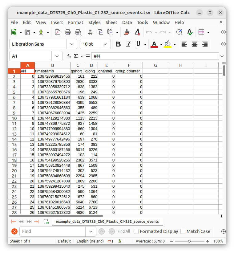
Fig. 3.9 Screenshot of LibreOffice Calc showing an events file of ABCD converted to ASCII.
Common spreadsheet software can easily open this file format (see Fig. 3.9).
Note
Events files do not directly contain the energy spectra, they are so called list mode files (i.e. files that contain all the events in the recording order). In order to generate spectra we need to analyze the events files with the available python scripts.
3.3.2. Plotting energy spectra
We can now plot the energy spectra associated with one of these files. Use the script:
user-tutorial@abcd-tutorial:~/abcd_tutorial$ plot_spectra.py -h
usage: plot_spectra.py [-h] [-n NS_PER_SAMPLE] [-w SMOOTH_WINDOW]
                       [-R ENERGY_RESOLUTION] [-e ENERGY_MIN] [-E ENERGY_MAX]
                       [-B BUFFER_SIZE] [-d] [-s] [--save_plot]
                       [--images_extension IMAGES_EXTENSION] [--disable_normalization]
                       file_names [file_names ...] channel

Plots multiple time normalized spectra from ABCD events data files.

positional arguments:
  file_names            List of space-separated file names
  channel               Channel selection (all or number)

options:
  -h, --help            show this help message and exit
  -n NS_PER_SAMPLE, --ns_per_sample NS_PER_SAMPLE
                        Nanoseconds per sample (default: 0.001953)
  -w SMOOTH_WINDOW, --smooth_window SMOOTH_WINDOW
                        Smooth window (default: 1.000000)
  -R ENERGY_RESOLUTION, --energy_resolution ENERGY_RESOLUTION
                        Energy resolution (default: 20.000000)
  -e ENERGY_MIN, --energy_min ENERGY_MIN
                        Energy min (default: 0.000000)
  -E ENERGY_MAX, --energy_max ENERGY_MAX
                        Energy max (default: 20000.000000)
  -B BUFFER_SIZE, --buffer_size BUFFER_SIZE
                        Buffer size for file reading (default: 167772160.000000)
  -d, --enable_derivatives
                        Enable spectra derivatives calculation
  -s, --save_data       Save histograms to file
  --save_plot           Save plot to file
  --images_extension IMAGES_EXTENSION
                        Define the extension of the image files (default: pdf)
  --disable_normalization
                        Disable the time normalization of the spectra
As usual it has a handy in-line help. This script calculates the energy spectra of events files with the given parameters and the selected channel. It is able to plot the result to an image, but also to save the result to a CSV file that can be read by something else (like spreadsheet software). First we plot the energy spectrum of a LaBr detector in channel 1:
user-tutorial@abcd-tutorial:~/abcd_tutorial$ plot_spectra.py -E 20000 --save_plot --images_extension=png example_data_DT5730_Ch1_LaBr3_Ch6_CeBr3_Ch7_CeBr3_coincidence_events.ade 1
Using buffer size: 167772160
Reading: example_data_DT5730_Ch1_LaBr3_Ch6_CeBr3_Ch7_CeBr3_coincidence_events.ade
    Reading chunk: 0
    Reading chunk: 1
    ERROR: min() arg is an empty sequence
    Total number of events of channel 1: 71167
    Number of events in energy range: 70285
    Time delta: 19863.900843 s
    Average rate total: 3.582730 Hz
    Average rate in range: 3.538328 Hz
Saving figure to: example_data_DT5730_Ch1_LaBr3_Ch6_CeBr3_Ch7_CeBr3_coincidence_events_ch1.png
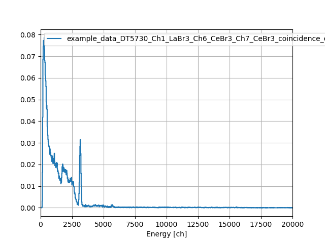
Fig. 3.10 Spectrum of the example data available in ABCD. It is the background spectrum of a LaBr detector.
Fig. 3.10 shows the resulting image generated by the script. We can now save the resulting spectrum to a CSV file:
user-tutorial@abcd-tutorial:~/abcd_tutorial$ plot_spectra.py -E 20000 -s example_data_DT5730_Ch1_LaBr3_Ch6_CeBr3_Ch7_CeBr3_coincidence_events.ade 1
Using buffer size: 167772160
Reading: example_data_DT5730_Ch1_LaBr3_Ch6_CeBr3_Ch7_CeBr3_coincidence_events.ade
    Reading chunk: 0
    Reading chunk: 1
    ERROR: min() arg is an empty sequence
    Total number of events of channel 1: 71167
    Number of events in energy range: 70285
    Time delta: 19863.900843 s
    Average rate total: 3.582730 Hz
    Average rate in range: 3.538328 Hz
    Writing qlong histogram to: example_data_DT5730_Ch1_LaBr3_Ch6_CeBr3_Ch7_CeBr3_coincidence_events_ch1_energy.csv
user-tutorial@abcd-tutorial:~/abcd_tutorial$ head -n 20 example_data_DT5730_Ch1_LaBr3_Ch6_CeBr3_Ch7_CeBr3_coincidence_events_ch1_energy.csv
# #energy,counts
0.000000000000000000e+00,0.000000000000000000e+00
2.000000000000000000e+01,0.000000000000000000e+00
4.000000000000000000e+01,0.000000000000000000e+00
6.000000000000000000e+01,0.000000000000000000e+00
8.000000000000000000e+01,0.000000000000000000e+00
1.000000000000000000e+02,4.027406330258181347e-04
1.200000000000000000e+02,3.070897326821863359e-03
1.400000000000000000e+02,1.636133821667386246e-02
1.600000000000000000e+02,4.178434067642863153e-02
1.800000000000000000e+02,6.866727793090199317e-02
2.000000000000000000e+02,7.455735968890458976e-02
2.200000000000000000e+02,7.727585896182885550e-02
2.400000000000000000e+02,7.450701710977634951e-02
2.600000000000000000e+02,7.727585896182885550e-02
2.800000000000000000e+02,7.858476601916276894e-02
3.000000000000000000e+02,7.324845263157067632e-02
3.200000000000000000e+02,6.796248182310681007e-02
3.400000000000000000e+02,6.710665797792694787e-02
3.600000000000000000e+02,6.121657621992435822e-02
3.3.3. Plotting Pulse Shape Discrimination diagrams
We can now move on to the Pulse Shape Discrimination (PSD) diagrams associated with one of these files. Use the script:
user-tutorial@abcd-tutorial:~/abcd_tutorial$ plot_PSD.py -h
usage: plot_PSD.py [-h] [-t PSD_THRESHOLD] [-n NS_PER_SAMPLE] [-w SMOOTH_WINDOW]
                   [-r PSD_RESOLUTION] [-p PSD_MIN] [-P PSD_MAX]
                   [-R ENERGY_RESOLUTION] [-e ENERGY_MIN] [-E ENERGY_MAX]
                   [-B BUFFER_SIZE] [-s] [--polygon_file POLYGON_FILE]
                   file_names [file_names ...] channel

Plots Pulse Shape Discrimination information from ABCD events data files.

positional arguments:
  file_names            List of space-separated file names
  channel               Channel selection (all or number)

options:
  -h, --help            show this help message and exit
  -t PSD_THRESHOLD, --PSD_threshold PSD_THRESHOLD
                        Simple PSD threshold for n/γ discrimination (default:
                        0.170000)
  -n NS_PER_SAMPLE, --ns_per_sample NS_PER_SAMPLE
                        Nanoseconds per sample (default: 0.001953)
  -w SMOOTH_WINDOW, --smooth_window SMOOTH_WINDOW
                        Smooth window (default: 1.000000)
  -r PSD_RESOLUTION, --PSD_resolution PSD_RESOLUTION
                        PSD resolution (default: 0.010000)
  -p PSD_MIN, --PSD_min PSD_MIN
                        PSD min (default: -0.100000)
  -P PSD_MAX, --PSD_max PSD_MAX
                        PSD max (default: 0.700000)
  -R ENERGY_RESOLUTION, --energy_resolution ENERGY_RESOLUTION
                        Energy resolution (default: 20.000000)
  -e ENERGY_MIN, --energy_min ENERGY_MIN
                        Energy min (default: 0.000000)
  -E ENERGY_MAX, --energy_max ENERGY_MAX
                        Energy max (default: 20000.000000)
  -B BUFFER_SIZE, --buffer_size BUFFER_SIZE
                        Buffer size for file reading (default: 167772160.000000)
  -s, --save_data       Save histograms to file
  --polygon_file POLYGON_FILE
                        Filename with a polygon to be drawn on top of the plot
This script calculates the energy spectra and the PSD diagram of events files. The PSD parameter is calculated according to:
Where \(Q_{\text{long}}\) and \(Q_{\text{short}}\) refer to the results of the two integration results over two intervals for the traditional double integration method for PSD.
\(Q_{\text{long}}\) and \(Q_{\text{short}}\) are the two Q entries in the processed events binary representation (see Section 7.2.2).
Also this script is able to plot the result to an image, but also to save the result to a CSV file.
Plot the PSD diagram first:
user-tutorial@abcd-tutorial:~/abcd_tutorial$ plot_PSD.py example_data_DT5725_Ch0_Plastic_Cf-252_source_events.ade 0
Using buffer size: 167772160
Reading: example_data_DT5725_Ch0_Plastic_Cf-252_source_events.ade
    Reading chunk: 0
/usr/bin/plot_PSD.py:179: RuntimeWarning: divide by zero encountered in true_divide
  PSDs = (qlongs.astype(np.float64) - qshorts) / qlongs
    Reading chunk: 1
    ERROR: min() arg is an empty sequence
    Number of events: 91952
    Time delta: 317.095820 s
    Average rate: 289.981748 Hz
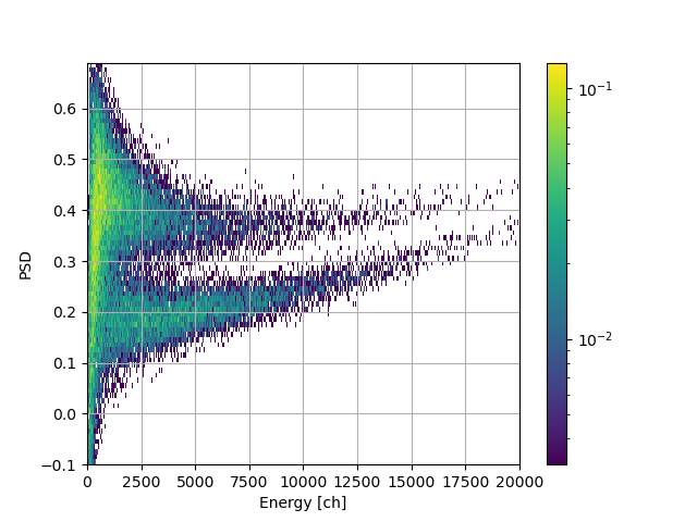
Fig. 3.11 Spectrum of the example data available in ABCD. It is the PSD diagram of a 252 Cf source detected with a plastic scintillation detector.
Fig. 3.11 shows the resulting image of the bidimensional histogram PSD parameter vs energy. The two data bananas represent the two populations of neutrons and gammas emitted by a 252 Cf source detected with a plastic scintillation detector. We can now save the energy spectrum and PSD distribution to CSV files:
user-tutorial@abcd-tutorial:~/abcd_tutorial$ plot_PSD.py -s example_data_DT5725_Ch0_Plastic_Cf-252_source_events.ade 0
Using buffer size: 167772160
Reading: example_data_DT5725_Ch0_Plastic_Cf-252_source_events.ade
    Reading chunk: 0
/usr/bin/plot_PSD.py:179: RuntimeWarning: divide by zero encountered in true_divide
  PSDs = (qlongs.astype(np.float64) - qshorts) / qlongs
    Reading chunk: 1
    ERROR: min() arg is an empty sequence
    Number of events: 91952
    Time delta: 317.095820 s
    Average rate: 289.981748 Hz
    Writing qlong histogram to: example_data_DT5725_Ch0_Plastic_Cf-252_source_events_qlong.csv
    Writing PSD histogram to: example_data_DT5725_Ch0_Plastic_Cf-252_source_events_PSD.csv
3.3.4. Studying timestamps
Timestamps are valuable not only to determine Time-of-Flights, but also to diagnose acquisitions and digitizer behavior. Plotting the sequence of timestamps shows how the timestamps evolve during an acquisition and can highlight some problems (see Fig. 3.12).
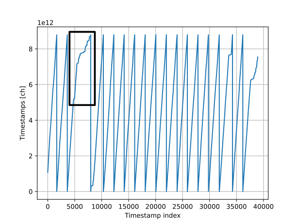
Fig. 3.12 Plot of the consecutive timestamps values. This plot shows two common issues related to the acquisition. In the black rectangle there is an area in which the slope of the timestamps changes. This change highlights a period of time in which the acquisition rate was changing. This regular saw pattern demonstrates that the timestamp in the digitizer was overflowing.
The plot of the timestamps values should be in general rising monotonically, because timestamps indicate the passing of time. On a very small scale there could be regions in which timestamps reduce their values, due to buffering effects in the digitizers and in the framework.
If there are changes in the slope it means that the acquisition rate changed during the acquisition. If the acquisition rate is roughly constant then the time delay between two consecutive events should be the same on the average. In this case the diagram slope shows the average delay. If the slope changes it means that the average delay is changing.
If the plot shows a saw pattern (Fig. 3.12), it means that the timestamp was resetting during the acquisition. There are several possible explanations:
The digitizer was reset during the acquisition for an error;
The timestamp was forcefully reset by the user;
The data file is an accumulation of several acquisitions and thus the digitizer was resetting in between them;
If the saw pattern is very regular, then it means that the timestamp was overflowing in the digitizer. This last issue can be fixed in post-processing.
To plot the sequence of timestamps, use the script:
user-tutorial@abcd-tutorial:~/abcd_tutorial$ plot_timestamps.py -n 0.001953125 -d 0.001 example_data_DT5730_Ch2_LaBr3_Ch4_LYSO_Ch6_YAP_events.ade 4 -h
usage: plot_timestamps.py [-h] [-n NS_PER_SAMPLE] [-N DELTA_BINS] [-d DELTA_MIN] [-D DELTA_MAX] [-B BUFFER_SIZE] [-s] file_names [file_names ...] channel

Plots multiple timestamps sequences and distributions of time differences from ABCD events data files.

positional arguments:
  file_names            List of space-separated file names
  channel               Channel selection (all or number)

options:
  -h, --help            show this help message and exit
  -n NS_PER_SAMPLE, --ns_per_sample NS_PER_SAMPLE
                        Nanoseconds per sample, if specified the timestamps are converted
  -N DELTA_BINS, --delta_bins DELTA_BINS
                        Number of bins in the time differences histogram (default: 1000)
  -d DELTA_MIN, --delta_min DELTA_MIN
                        Minimum time difference (default: 0.000000)
  -D DELTA_MAX, --delta_max DELTA_MAX
                        Maximum time difference, if not specified the absolute maximum is used
  -B BUFFER_SIZE, --buffer_size BUFFER_SIZE
                        Buffer size for file reading (default: 167772160.000000)
  -s, --save_data       Save histograms to file
We can check the an example data file:
user-tutorial@abcd-tutorial:~/abcd_tutorial$ plot_timestamps.py -n 0.001953125 -d 0.001 example_data_DT5730_Ch2_LaBr3_Ch4_LYSO_Ch6_YAP_events.ade 4
Using buffer size: 167772160
Reading: example_data_DT5730_Ch2_LaBr3_Ch4_LYSO_Ch6_YAP_events.ade
    Reading chunk: 0
    Reading chunk: 1
    ERROR: min() arg is an empty sequence
    Number of events: 90287
    Time interval: [0.00162634, 689.395] s
    Time delta: 689.394 s
    Measured rate: 130.966 1/s
    True rate: 103.35 1/s
    Dead time: -0.00204032 s (-0.000296%)
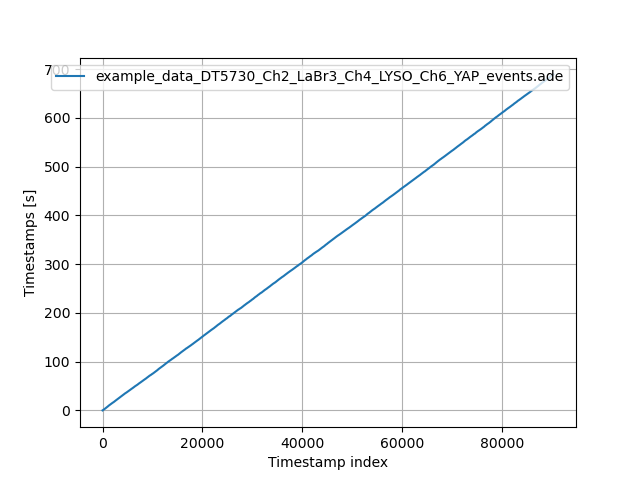
Fig. 3.13 Plot of the consecutive timestamps values of an example file.
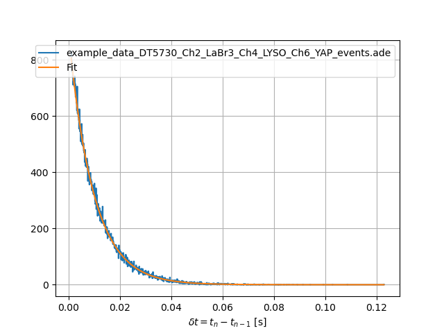
Fig. 3.14 Plot of the histogram of the time differences between consecutive events in an example file.
Fig. 3.13 shows the resulting timestamps sequence of the examples file. In this case the plot is monotonic and shows no particular issues.
Studying the time difference between two consecutive events can give information about the true activity of the source. Assuming a Poissonian statistics, it is possible to determine the average emission rate of a source by determining the decay time of the histogram of the time differences. If the average rate does not correspond to the calculation of the number of events seen in the acquisition time, it probably means that the deadtime of digitizer was significant. The aforementioned script does this calculation and plots the result (Fig. 3.14). In order to do this calculation it is necessary to know the conversion factor between the timestamps values and nanoseconds. For the specific case of the shown example data, the two acquisition rates match:
user-tutorial@abcd-tutorial:~/abcd_tutorial$ plot_timestamps.py -n 0.001953125 -d 0.001 example_data_DT5730_Ch2_LaBr3_Ch4_LYSO_Ch6_YAP_events.ade 4
Using buffer size: 167772160
Reading: example_data_DT5730_Ch2_LaBr3_Ch4_LYSO_Ch6_YAP_events.ade
    Reading chunk: 0
    Reading chunk: 1
    ERROR: min() arg is an empty sequence
    Number of events: 90287
    Time interval: [0.00162634, 689.395] s
    Time delta: 689.394 s
    Measured rate: 130.966 1/s
    True rate: 103.35 1/s
    Dead time: -0.00204032 s (-0.000296%)
3.3.5. Dependency of the energy spectrum on time
Another interesting application of timestamps is to study the evolution of the energy spectrum over time. Over long acquisition runs a detector might show some gain drifts, due to several reasons. Gain drifts might produce a worse resolution on the spectrum, that can be corrected offline. There could also be apparent rate changes, because with different gains more noise could pass the energy threshold. We can check with the script:
user-tutorial@abcd-tutorial:~/abcd_tutorial$ plot_Evst.py -h
usage: plot_Evst.py [-h] [-n NS_PER_SAMPLE] [-N EVENTS_COUNT] [-r TIME_RESOLUTION] [-t TIME_MIN] [-T TIME_MAX] [-R ENERGY_RESOLUTION] [-e ENERGY_MIN] [-E ENERGY_MAX] [--save_plots]
                    [--images_extension IMAGES_EXTENSION]
                    file_name channel

Plot the time dependency of the energy spectrum from ABCD events data files.

positional arguments:
  file_name             Input file name
  channel               Channel selection (all or number)

options:
  -h, --help            show this help message and exit
  -n NS_PER_SAMPLE, --ns_per_sample NS_PER_SAMPLE
                        Nanoseconds per sample (default: 0.001953)
  -N EVENTS_COUNT, --events_count EVENTS_COUNT
                        Maximum number of events to be read from file, if -1 then read all events (default: -1.000000)
  -r TIME_RESOLUTION, --time_resolution TIME_RESOLUTION
                        Time resolution (default: 2.000000)
  -t TIME_MIN, --time_min TIME_MIN
                        Time min (default: -1.000000)
  -T TIME_MAX, --time_max TIME_MAX
                        Time max (default: -1.000000)
  -R ENERGY_RESOLUTION, --energy_resolution ENERGY_RESOLUTION
                        Energy resolution (default: 20.000000)
  -e ENERGY_MIN, --energy_min ENERGY_MIN
                        Energy min (default: 0.000000)
  -E ENERGY_MAX, --energy_max ENERGY_MAX
                        Energy max (default: 66000.000000)
  --save_plots          Save plots to file
  --images_extension IMAGES_EXTENSION
                        Define the extension of the image files (default: pdf)
This script needs to know the conversion factor between the timestamps and nanoseconds, in order to determine the real time scale. We can run it on the example data:
user-tutorial@abcd-tutorial:~/abcd_tutorial$ plot_Evst.py -n 0.001953125 --save_plots --images_extension=png -r 100 -R 10 -e 0 -E 4000 example_data_DT5730_Ch1_LaBr3_Ch6_CeBr3_Ch7_CeBr3_coincidence_events.ade 1
### ### Reading: example_data_DT5730_Ch1_LaBr3_Ch6_CeBr3_Ch7_CeBr3_coincidence_events.ade
Energy min: 0.000000 ch
Energy max: 4000.000000 ch
N_E: 400
Time min: 0.145500 s
Time max: 19864.046343 s
Time delta: 19863.900843 s
N_t: 198
Saving plot to: example_data_DT5730_Ch1_LaBr3_Ch6_CeBr3_Ch7_CeBr3_coincidence_events_Ch1_Evst.png
Saving plot to: example_data_DT5730_Ch1_LaBr3_Ch6_CeBr3_Ch7_CeBr3_coincidence_events_Ch1_Rvst.png
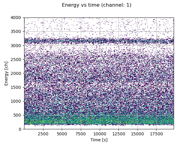
Fig. 3.15 Plot of the dependency of the energy spectrum on the time in an example file.
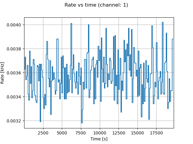
Fig. 3.16 Plot of the dependency of the acquisition rate on the time in an example file.
Fig. 3.15 and Fig. 3.16 show the results of the dependency of the energy spectrum and acquisition on the example data file.
3.3.6. Calculating Time-of-Flights
It is also possible to calculate the Time-of-Flight (ToF) between detectors in saved events files, using the script:
user-tutorial@abcd-tutorial:~/abcd_tutorial$ plot_ToF.py -h
usage: plot_ToF.py [-h] [-n NS_PER_SAMPLE] [-r TIME_RESOLUTION] [-t TIME_MIN] [-T TIME_MAX] [-R ENERGY_RESOLUTION] [-e ENERGY_MIN] [-E ENERGY_MAX] [--reference_energy_min REFERENCE_ENERGY_MIN]
                   [--reference_energy_max REFERENCE_ENERGY_MAX] [-d PSD_RESOLUTION] [-p PSD_MIN] [-P PSD_MAX] [--reference_PSD_min REFERENCE_PSD_MIN] [--reference_PSD_max REFERENCE_PSD_MAX] [-B BUFFER_SIZE]
                   [-s] [--save_plots] [-m TOF_MODULO] [-o TOF_OFFSET] [--images_extension IMAGES_EXTENSION]
                   file_name channel_a channel_b

Reads an ABCD events file and plots the ToF between two channels

positional arguments:
  file_name             Input file name
  channel_a             Channel selection
  channel_b             Channel selection

options:
  -h, --help            show this help message and exit
  -n NS_PER_SAMPLE, --ns_per_sample NS_PER_SAMPLE
                        Nanoseconds per sample (default: 0.001953)
  -r TIME_RESOLUTION, --time_resolution TIME_RESOLUTION
                        Time resolution (default: 2.000000)
  -t TIME_MIN, --time_min TIME_MIN
                        Time min (default: -200.000000)
  -T TIME_MAX, --time_max TIME_MAX
                        Time max (default: 200.000000)
  -R ENERGY_RESOLUTION, --energy_resolution ENERGY_RESOLUTION
                        Energy resolution (default: 20.000000)
  -e ENERGY_MIN, --energy_min ENERGY_MIN
                        Energy min (default: 0.000000)
  -E ENERGY_MAX, --energy_max ENERGY_MAX
                        Energy max (default: 66000.000000)
  --reference_energy_min REFERENCE_ENERGY_MIN
                        Reference energy min (default: 0.000000)
  --reference_energy_max REFERENCE_ENERGY_MAX
                        Reference energy max (default: 66000.000000)
  -d PSD_RESOLUTION, --PSD_resolution PSD_RESOLUTION
                        PSD resolution (default: 0.010000)
  -p PSD_MIN, --PSD_min PSD_MIN
                        PSD min (default: -0.100000)
  -P PSD_MAX, --PSD_max PSD_MAX
                        PSD max (default: 0.700000)
  --reference_PSD_min REFERENCE_PSD_MIN
                        Reference PSD min (default: -0.100000)
  --reference_PSD_max REFERENCE_PSD_MAX
                        Reference PSD max (default: 0.700000)
  -B BUFFER_SIZE, --buffer_size BUFFER_SIZE
                        Buffer size for file reading (default: 16777216.000000)
  -s, --save_data       Save histograms to file
  --save_plots          Save plots to file
  -m TOF_MODULO, --ToF_modulo TOF_MODULO
                        If set, the ToF is calculated modulo this value
  -o TOF_OFFSET, --ToF_offset TOF_OFFSET
                        If a modulo is set, an offset added to the ToF in ns (default: 0.000000)
  --images_extension IMAGES_EXTENSION
                        Define the extension of the image files (default: pdf)
The script uses the same algorithm of the tofcalc module to determine the time difference between pulses from two different detectors (for more information see: Section 13).
The script needs to know the conversion factor between the timestamp values and nanoseconds.
Launch the script as:
user-tutorial@abcd-tutorial:~/abcd_tutorial$ plot_ToF.py --save_plots --images_extension=png -n 0.001953125 -r 0.25 -t -80 -T -40 -E 7000 --reference_energy_max 3000 -P 1.0 --reference_PSD_max 1.0 example_data_DT5730_Ch1_LaBr3_Ch6_CeBr3_Ch7_CeBr3_coincidence_events.ade 1 6
Using buffer size: 16777216
Energy min: 0.000000
Energy max: 7000.000000
N_E: 350
Reference energy min: 0.000000
Reference energy max: 3000.000000
N_E: 150
Time min: -80.000000
Time max: -40.000000
N_t: 160
Time modulo: 0.000000
Time offset: 0.000000
PSD min: -0.100000
PSD max: 1.000000
N_PSD: 110
Reference PSD min: -0.100000
Reference PSD max: 1.000000
N_PSD: 110
### ### Reading chunk: 0
Selecting channels...
Sorting data...
Number of events: 113720
Time delta: 38.796681 s
Average rate: 2931.178546 Hz
Starting the main loop for 113720 events...
selected_events: 55456 / 113720 (48.77%)
Total time: 0:00:00.732470; time per event: 6.440995 µs
### ### Reading chunk: 1
Selecting channels...
Sorting data...
Number of events: 0
    Number of events: 113720
    Time delta: 38.796681 s
    Average rate: 2931.178546 Hz
Saving plot to: example_data_DT5730_Ch1_LaBr3_Ch6_CeBr3_Ch7_CeBr3_coincidence_events_Ch1andCh6_E-histos.png
Saving plot to: example_data_DT5730_Ch1_LaBr3_Ch6_CeBr3_Ch7_CeBr3_coincidence_events_Ch1andCh6_E-ToF-histos.png
Saving plot to: example_data_DT5730_Ch1_LaBr3_Ch6_CeBr3_Ch7_CeBr3_coincidence_events_Ch1andCh6_PSD-ToF-histos.png
Saving plot to: example_data_DT5730_Ch1_LaBr3_Ch6_CeBr3_Ch7_CeBr3_coincidence_events_Ch1andCh6_E-E-histo.png
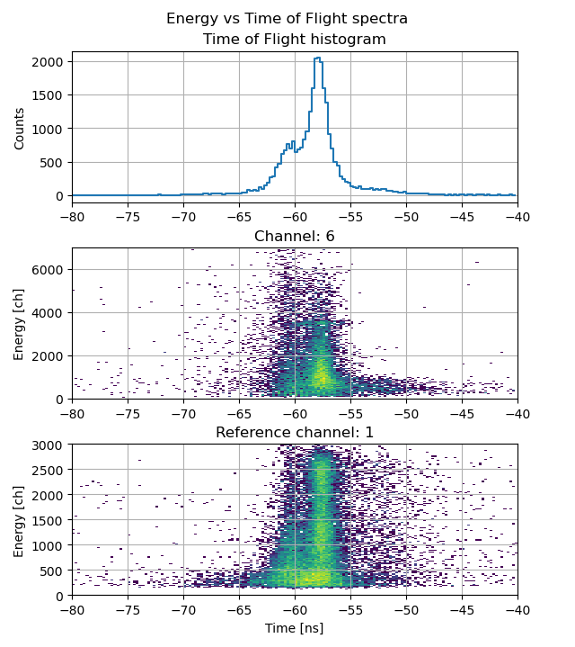
Fig. 3.17 Plot of the dependency of the detected energies on the Time-of-Flight in an example file. The reference detector is a LaBr. The other detector is a CeBr detecting the intrinsic radioactivity of the LaBr.
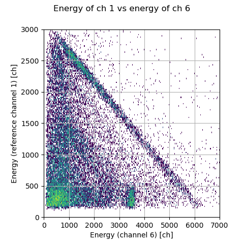
Fig. 3.18 Plot of the relationship between the detected energies in temporal coincidence in an example file. The reference detector is a LaBr. The other detector is a CeBr detecting the intrinsic radioactivity of the LaBr.
Fig. 3.17 and Fig. 3.18 show the results of the ToF analysis on the example data file. These plots match the plots calculated on-line in the previous tutorial. An attentive reader might notice that the energies have different values. Indeed the events file that we just analyzed with the script was calculated on-board by the digitizer. The digitizer firmware analyzed the waveforms and provided the processed events. In the previous tutorial we used a replay of the raw data, which contains also the waveforms. During the replay, the waveforms are reanalyzed by the waveforms analysis module of ABCD, which has a configuration that is a little bit different.
3.3.7. Waveforms displaying
We conclude this tutorial by plotting saved waveforms in an example waveforms file. Use the script:
user-tutorial@abcd-tutorial:~/abcd_tutorial$ plot_waveforms.py -h
usage: plot_waveforms.py [-h] [-c CHANNEL] [-n WAVEFORM_NUMBER] [--clock_step CLOCK_STEP] file_name

Plots waveforms from ABCD waveforms data files. Pressing the left and right keys shows the previous or next waveform. Pressing the up and down keys jump ahead or behind of 10 waveforms, page up and down jump
100 waveforms. Pressing the 'h' key resets the view to the full waveform. Pressing the 'f' key toggles between showing the waveform and its Fourier transform. Pressing the 'e' key exports the current waveform
to a CSV file.

positional arguments:
  file_name             Waveforms file name

options:
  -h, --help            show this help message and exit
  -c CHANNEL, --channel CHANNEL
                        Channel selection
  -n WAVEFORM_NUMBER, --waveform_number WAVEFORM_NUMBER
                        Plots the Nth waveform
  --clock_step CLOCK_STEP
                        Step of the ADC sampling of the waveform in ns (default: 2 ns)
This script generates an interactive plot of the waveforms allowing the user to go through the saved waveforms (see Fig. 3.19). It can also calculate the Fourier transform of the currently displayed waveform (see Fig. 3.20).
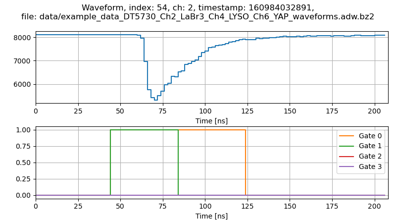
Fig. 3.19 Display of a waveform saved in an example file.
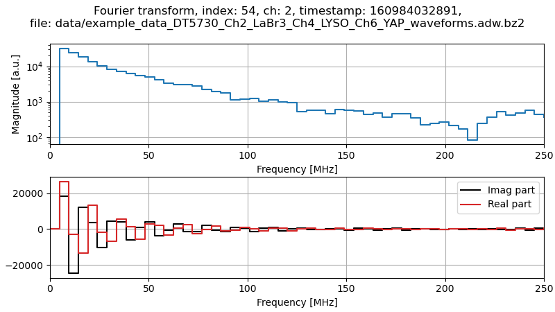
Fig. 3.20 Display of the Fourier transform of the waveform of Fig. 3.19.
Congratulations, again! With these plots we conclude this second tutorial. We just had an overview of the provided analysis programs, that can give a base on which new users can write their own analysis routines.